Making a geological map with Macrostrat and ggplot

Geological maps are important to include as figures in many papers. Often creating them can rely on existing figures or shapefiles that are in GIS. The Macrostrat database contains shapefiles for many Formations that can be returned using the API.

First we load the important packages. We will use data from Natural Earth to create the basemap. We also use a few other tools to get data from Macrostrat database and convert it to a simple feature (sf) object.

library(ggplot2)
library(sf)

## Linking to GEOS 3.9.0, GDAL 3.2.1, PROJ 7.2.1

library(ggspatial)
library(rnaturalearth)
library(rnaturalearthdata)
library(geojsonsf)
library(RCurl)

We load the state outlines for the map using this code.

South_base <- ne_states(country = "united states of america", returnclass = "sf")

Here we get data from Macrostrat. To change this to your formation of interest, use the sift interface to search for a unique strat_name_id for a formation of interest.

The data are then converted to a wkt and finally an sf object.

y <- getURL("https://macrostrat.org/api/v2/geologic_units/map?strat_name_id=2683&format=geojson_bare",
            .opts = curlOptions(ssl.verifypeer=FALSE, verbose=TRUE))
            
sf_temp <- geojson_wkt(y)

sf_map <- st_as_sf(sf_temp, wkt = 'geometry', crs = 4326) 

We then use ggplot to build the map.

First, we can create just the simple background base map.

ggplot(data = South_base) +
  geom_sf()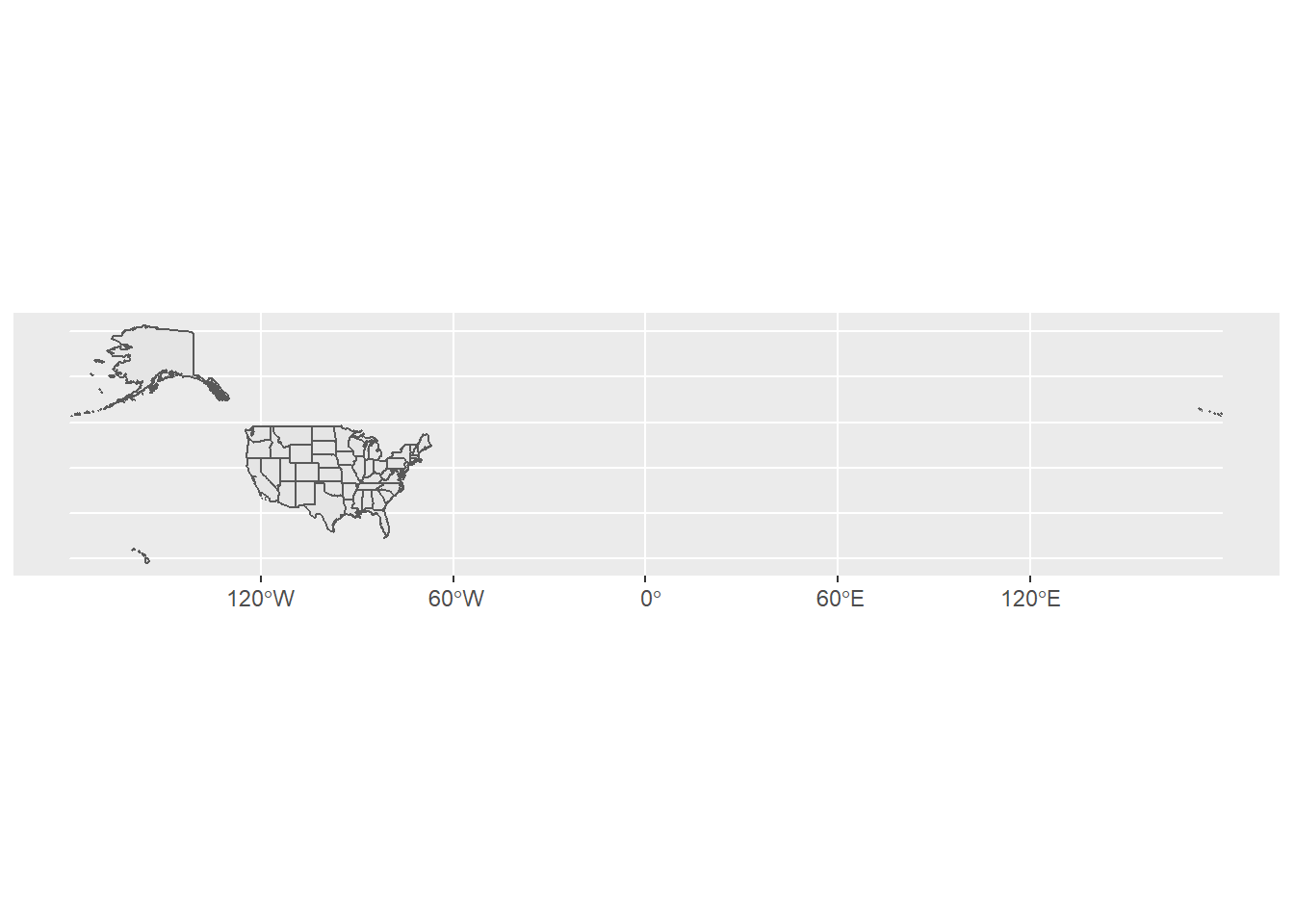

Then we can add the geological data.

ggplot(data = South_base) +
  geom_sf()+
  geom_sf(data = sf_map,
          color = "#A6D84A",
          fill = "#A6D84A",
          alpha = .5)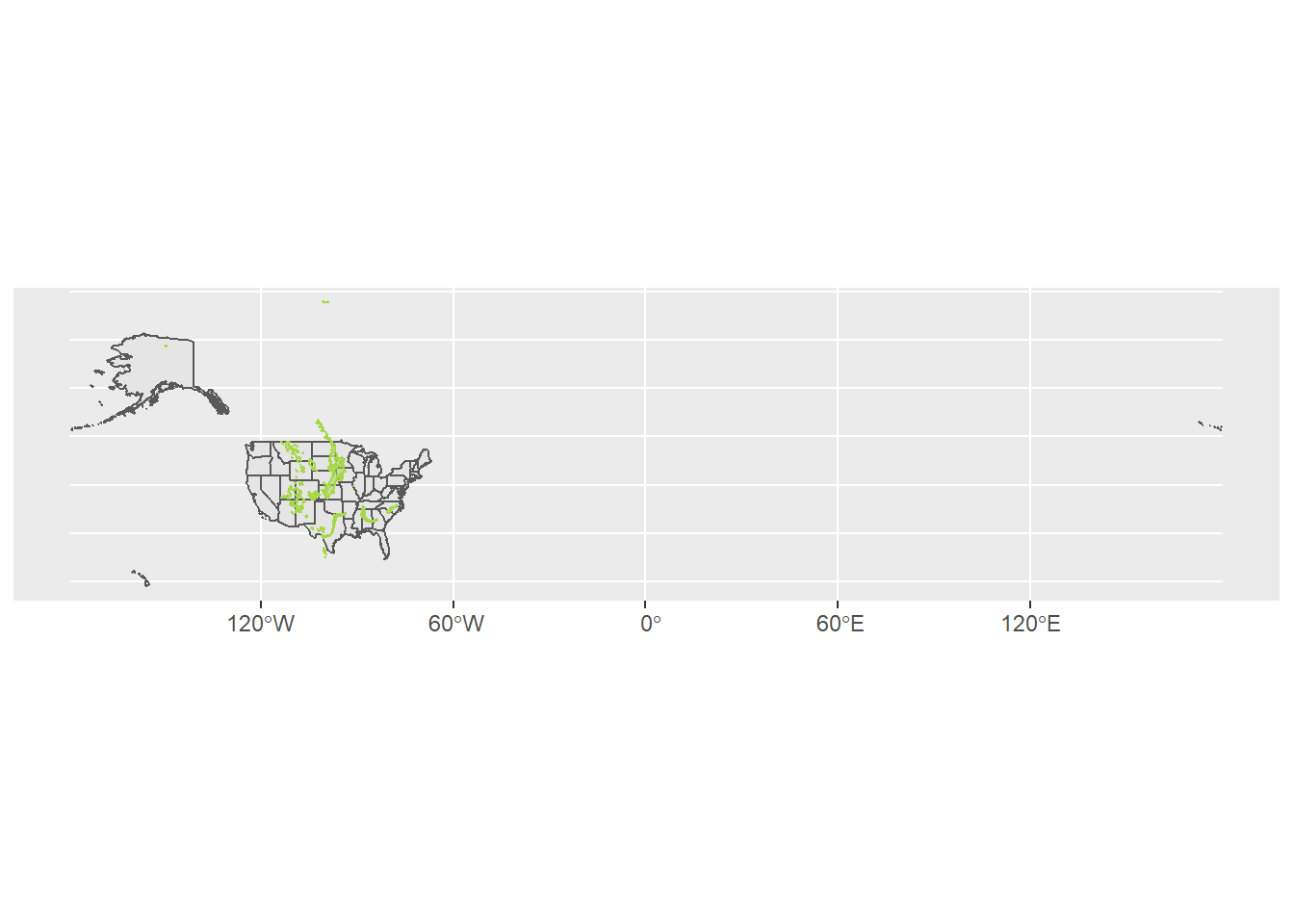

Next we can select a smaller area and then add a North arrow.

ggplot(data = South_base) +
  geom_sf()+
  geom_sf(data = sf_map,
          color = "#A6D84A",
          fill = "#A6D84A",
          alpha = .5)+
  coord_sf(xlim = c(-90, -82), ylim = c(28, 37.5), expand = FALSE)+
  annotation_north_arrow(location = "bl", which_north = "true", 
                         pad_x = unit(0.75, "in"), pad_y = unit(0.5, "in"),
                         style = north_arrow_fancy_orienteering)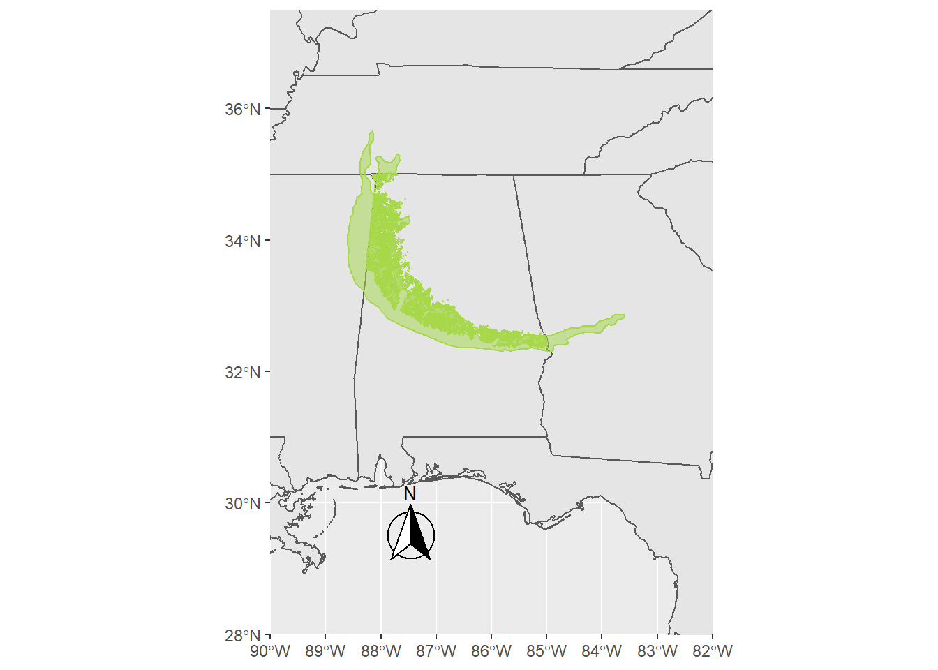

Finally, we add a scale bar, background colors, dashes, and fill the ocean with a light blue.

ggplot(data = South_base) +
  geom_sf()+
  geom_sf(data = sf_map,
          color = "#A6D84A",
          fill = "#A6D84A",
          alpha = .5)+
  coord_sf(xlim = c(-90, -82), ylim = c(28, 37.5), expand = FALSE)+
  annotation_north_arrow(location = "bl", which_north = "true", 
                         pad_x = unit(0.75, "in"), pad_y = unit(0.5, "in"),
                         style = north_arrow_fancy_orienteering)+
    annotation_scale(location = "bl", width_hint = 0.5) +
  theme(panel.grid.major = element_line(color = gray(.5),
                                        linetype = "dashed",
                                        size = 0.5),
        panel.background = element_rect(fill = "aliceblue"))+
        theme_bw()

## Scale on map varies by more than 10%, scale bar may be inaccurate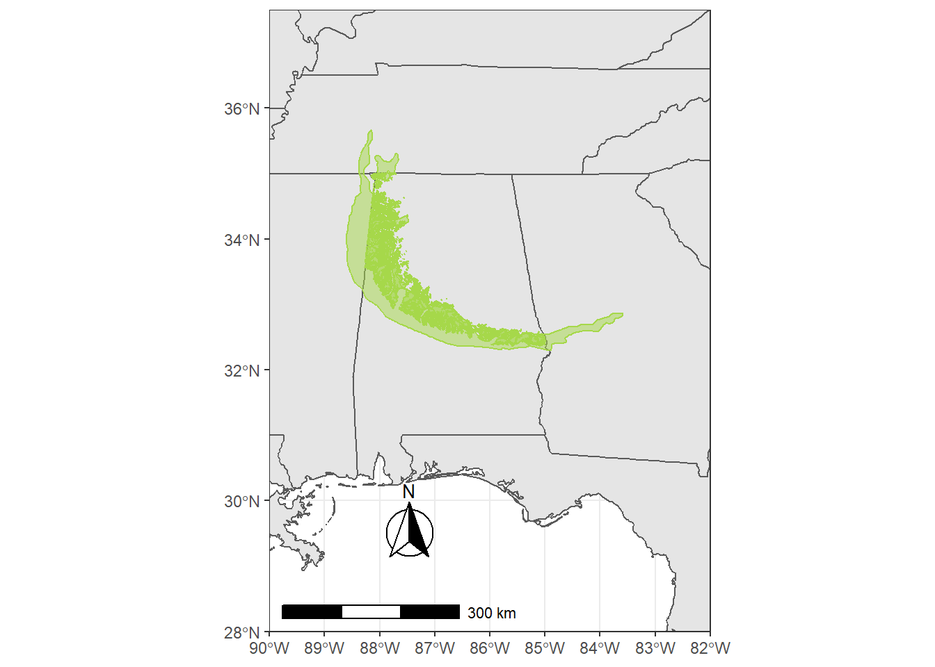

And there you have a map of a geological unit overlain on a state map in R.